A Numerical Example in Polytree

A Numerical Example 

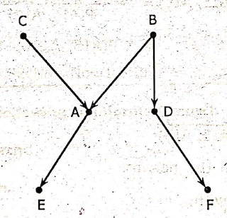
Let us consider a small polytree to explain the use of evidence above and evidence 

Fig. 3.8.2 A Small Polytree 

The probabilities that we take as given are, 

                P(C) =, 0.02 

                P(B) = 0.04 

                P(A| C, B) = 0.9 

                P(A, C, ᆨB) = 0.7 

                P(A | ᆨC, B) = 0.95 

                P(A | ᆨC, ᆨB) = 0.03 

                P(D | B) = 0.8 

                P(D | ᆨB) = 0.05 

                P(F | D) = 0.65 

                P(E | A) = 0.4 

                P(F | ᆨD) = 0.2 

                P(E | ᆨA) = 0.6 

We have to calculate P(B | E) first of all, we apply Bayes rule, 

                P(B | E) = KP(E | B) P(B) 

here, 

                

For calculating P(E | B) we apply top-down algorithm,

                

                

                P(A | B) = P(A | C, B) P(C) + P(A | ᆨC, B) P(ᆨC)

                P(A | B) = 0.949

                = 0.9 x 0.02 + 0.95 x 0.98 

                =0.018 + 0.931 = 0.949 

                P(A | B) = 0.949 

                P(ᆨA | B) = 0.051 

                P(E | B) = P(E | A) x 0.949 + P(E | ᆨA),x 0.051 

                = 0.4 x 0.949 + 0.6 x 0.051 

                P(E | B) = 0.4102 

                P(ᆨE | B) = 0.5898.

                P(B | E) = K P(E | B) P(B) 

                = K x 0.4102 x. 0.04

                = K x 0.016 

                = K P(E | ᆨB) P(ᆨB)

 

                

                

                = P(A | C, ᆨB) P(C) + P(A | ᆨC, ᆨB)P(ᆨC) 

                = 0.7 x 0.02 + 0.03 x 0.98 

                = 0.014 + 0.0294 = 0.0434 

P(ᆨA | ᆨB) = 0.9566 

P(E | ᆨB)  = P(E | A) x 0.0434 + P(E | ᆨA) x 0.9566 

= 0.4 x 0.0434 + 0.6 x 0.9566 

= 0.01736 + 0.57396 

= 0.59132 

P(ᆨB | E) =K x 0.59132 x 0.96 

= K x 0.5676 

∴ P(B | E) + P(ᆨB | E) = 1 

0.016 K + 0.5676 K = 1

0.5836 K = 1 

 = 1.71 

∴ P(B | E) = 0.06 x 1.71 

= 0.02736 

Finally the probability of B given E is 0.02736 and K is 1.71. 

Bucket Elimination 

It is a method which is used to eliminate the sub-calculation which are repeated in the calculation.

If the network is not a polytree, the recursive procedures does not end.

Monte Carlo Method:

It is a method, which is used in the complicated networks where the recursive procedures does not end.

1. In this method the random values, are assigned to the parentless nodes using their marginal probabilities. 
2. The random values are assigned to the descendants by using conditional probability tables and this continues till the network is ended.
3. Every node in the network finally has a value.
4. P(B | E) can be estimated after a number. of trails.

Clustering 

This is another method where the nodes in the network are grouped into 'supernodes'.

1. These 'supernodes' are grouped in a way that, the graph of them forms a polytree. 
2. The combination of the values of the components of a supernode forms its values. 
3. Now these supernodes are considered to be the nodes of a polytree and the algorithms that are applied to a polytree are applied to them. 
4. But, being the combination of many nodes the supernodes may contain many conditional probability tables which gives the conditional probabilities of all the values of the supernodes which are conditioned on all the values of the parent nodes. The parent node may be a supernode again. This may again make the method complex.