Probabilistic Inference in Polytrees

PROBABILITIC INFERENCE IN POLYTREES 

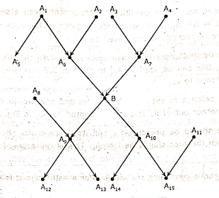
• A polytree is a network in which there exists a node B such that some of the nodes are connected to it only through its parents. 
• The nodes which are not connected by its parents are connected by its immediate successors. 
• The nodes connected by parents are said to be above B. 
• The nodes connected by its children are said to be below B. 
• It has to be noted that in the polytree this B node is the only path between the above nodes and below nodes. 
• The polytree network is shown in the Fig. 3.8.1.

Fig. 3.8.1 A Typical Polytree

Every node of the polytree has the same rules. 

Evidence Above 

    If all evidence nodes are above Q. We calculate P(B | A5, A4) as an example. . Here, bottom up recursive algorithm is used.

It is used to know the probability of every ancestor of B, if the evidence is given and till we reach the evidence or the evidence is below the ancestor.

The algorithm is as follows,. 

1) The parents of node B are taken, 

        

        (Here the summation is used to mention the four combinations, one is what is present i e.,  A6, A7, second one is substituting ᆨA6 for A6, the other is substituting ᆨA7 for A7, and other is substituting ᆨA6. and- ᆨA7). 

2) Conditional independence is used make the parents of Q as part of the evidence. 

        

3) Substituting this in first step gives, 

        

4) As the node is conditionally independent of non descendants if it parents are given, 

        

5) By using D-separation we can split the parents, 

        

6) As it is allowed by D-separation we ignore the evidence which is above one parent while we are calculating the probability of another parent, 

        

In the above equation P(B | A6, A7) is the probability, of the query node, where the value of its parents are given. 

P(A6 | A5) and P(A7 | A4) are the probabilities of the parents if the part of the evidence above the parent is given. 

The recursive process of algorithm continues till we reach the node which has the evidence node as a parent. 

In P(A7 | A4) the A4 node is the evidence node and it is the parent of A7.

Now the parents are involved. 

Since, 

        P(A7,  A3 | A4) = P(A7 | A3, A4) P(A3 | A4) 

Then, 

        

        

In P(A1 | A5) calculation we have, 

        

As in P(A1 | A5) the evidence node is note above the query node this recursive procedure is terminated and. as it is below evidence below method has to be used.

Bayes rule can also be used' to Obtain P(Al | A5) 

        

Now we can calculate P(A6 | A5) and then P(Q | A5, A4). 

Evidence Below

To calculate P(B | Al2, A13, A14, A11), as all the evidence nodes are below evidence below is used. 

Reasoning with Uncertain Information 

The algorithm used here is also a recursive algorithm. 

In this algorithm first we use Bayes rule. 

        

Let, 

        

Now D-Separation is used. 

I({Al2, A13}, {A14, A11) | Q)

which gives, 

        P(B | Al2, A13, A14, A11) = KP(Al2, A13 | B) P(A14, A11 | B) P(B) 

Now as there is a single evidence node B we use top-down recursive algorithm instead of bottom-up approach. 

As A9 is the present of Al2, A13 

P(Al2, A13, A9 | B) = P(Al2, A13 | A9, Q) P(A9 | B) 

which is from the definition of conditional independence. So the equation becomes, 

        

By using D-Separation, 

        I{Al2, A13}, B | A9) 

SO, 

        

P(A9 | B) can calculated by the parents involved in it, 

        

The value of P(A9 | A8, B) is given by the network.

Now P(Al2, A13 | A9) has to be calculated in the same recursive fashion from top to down. 

The recursive call stops after one step as the children of A9 i.e. Al2 and A13 are evidence nodes because, and Al2 and A13 are independent if A9 is given. 

Now, 

        P(A12, A13 | A9) = P(A12 | A9) P(A13 | A9) 

Now we calculate P(A14, Al1 |  B) by using top-down, procedure, 

        

        

        

                                                                                                                [∴ I(A14, All A10)] 

In the above expression the value of the middle term is not given directly.

So, we calculate P(A11 | A10) by top-down approach, 

        

        

In P(A11 | A15, A10). All is above the evidence nodes, so we have to use evidence above at this node. Now we use Bayes rule, 

        

Here, 

        

and P(M1) is given in the network. 

The algorithm. stops with, 

        P(A15, A10 | A11.) = P(A15 | A10, A11) P(A10 | A11) 

        

        P(A15, A10 | A11.) = P(A15 | A10, A11) P(A10) 

as A10 and Al1 are independent of each other. 

Finally all the results are combined. and K and K1 are calculate to find the solution to 

        P(B | Al2, A13, A14, A11). 

Evidence above and evidence below algorithms have a linear complexity in the number of nodes present in the network. 

Evidence Above and Below 

If we have evidence above 'B' and below 'B' like, 

                P(B | {A5, A4}, {Al2, A13, A14, A11})

then the evidences are separated into above denoted by    and below as .

Now, Bayes rule is used to write, 

                

Now, we use   as a factor of normalization. 

The equation becomes, 

                 

In can be noted that and  and  are d-separated by B, so

                

These probabilities can be got from evidence above and evidence below and    can be calculated.